I sometimes think the concept of espresso exists to trick us into thinking that perfection can exist, only to have reality handed to us on a plate to humble us. That’s the best way I can summarize the events that led to this post.

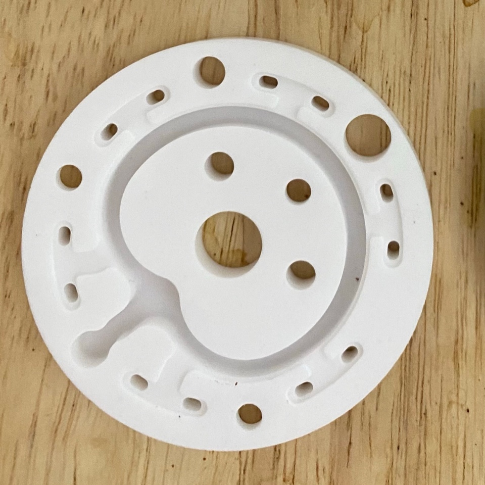
As the photo above might tell you, I stuck a temperature probe inside a puck. The decision wasn’t an easy one. I had to sacrifice a basket (although it wasn’t a basket I was using much anymore due to its insufficient hole coverage, despite it being a precision basket). The problem is though, you are essentially creating a channel in the puck. For the shots that I pulled over the course of this experiment, I don’t think I can say that the extent or behavior of the channel could be controlled to the extent I would have desired. However, my main motivation here was to measure temperature at different heights in a puck. We will however revisit this channeling behavior later in the post to improve the accuracy of the temperature behavior.

So you poked an espresso puck

Here’s what was done to collect data for this experiment:

1. An 2 mm hole was drilled in an 18g precision basket.
2. A probe was inserted at the bottom of the puck and flattened. 18g of coffee was then deposited, gently WDT’d and tamped with a Deccent V4 tamper (I used a non-calibrated leveling tamper on purpose to be able to control tamping force). A puck screen was placed atop the puck and a shot was pulled.
3. For the next shot, 4.5g coffee was first placed in the basket, the probe flattened in a way that it is level with the 4.5g slice when tamped. The coffee was gently raked and tamped along with the probe. The rest 13.5g was then deposited, gently WDT’d and firmly tamped. Puck screen was placed and shot was pulled.
4. This was done for the probe placed at bottom, 25% above bottom (4.5), 50% above bottom (9g), 75% above bottom (13.5g), below puck screen (18g) and top of puck screen.
5. Six such shots were pulled for for types of shots – Turbo shot, Extractamundo Dos!, Traditional 1:2 shot in 30s, Rao’s blooming espresso (slightly modified to induce a temperature decline).
6. Shot data was collected using a DE1 whereas probe temperature data was logged using a Yoctupuce thermocouple set to record every 0.25 seconds.

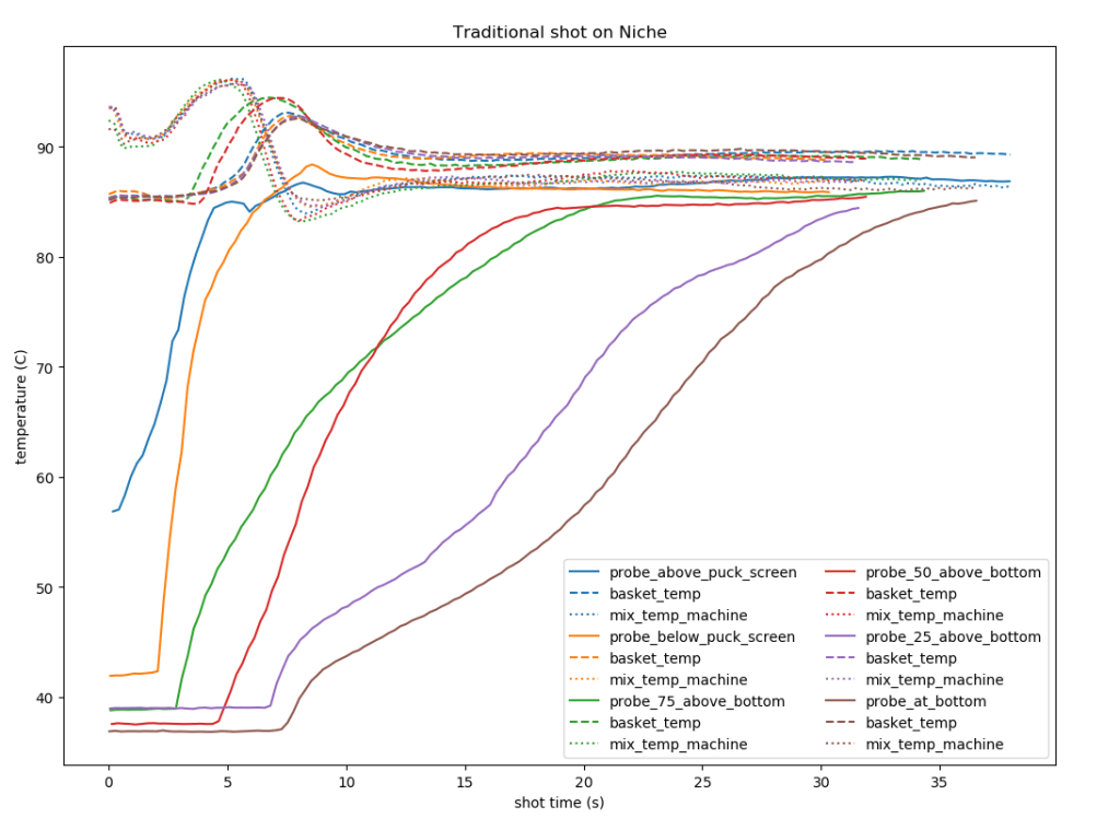
Some additional caveats about my particular setup before we dive into the plots. I have talked at length before how the DE1 needs unusually lower temperatures than other machines, a phenomenon that is only exacerbated due to my usage of prototype low thermal mass teflon grouphead parts. To give a tl;dr version of how a shot starts on my particular machine – the firmware seems to inject cold water at the start based on the temperature it records and assuming it’s to cool the stock brass parts to target temperature. However, in reality since the thermal mass is much lower in my case, the start temperature plummets. I compensate for this by starting my shot about 5C higher than the intended temperature, just so the average temperature by the time the puck saturates is within spec. You’ll see this phenomenon in the “basket_temp” plots that will be presented below. basket_temp in case of the DE1 is the sensor that sits in the dispersion block right above the shower screen, i. e. a k-type probe is placed in the machine right above the puck that measures the temperature that’s a mix of the teflon dispersion block itself and the water passing through it.

So, what’s really being measured?

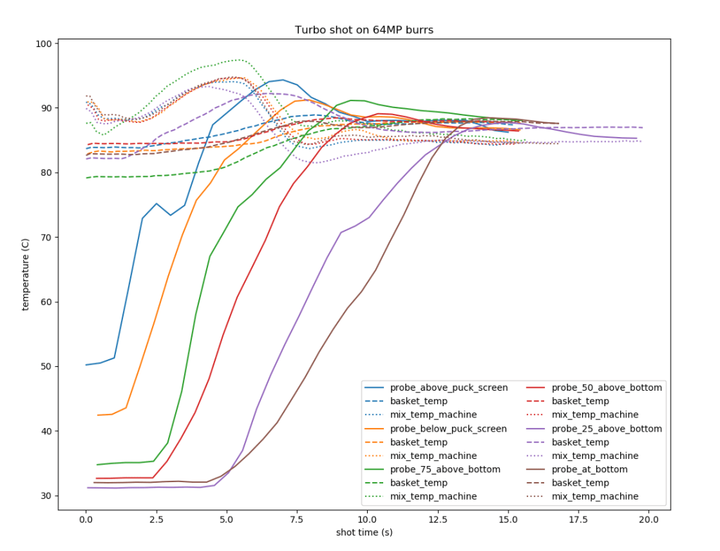
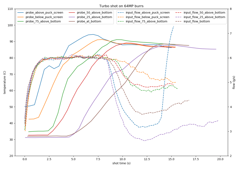
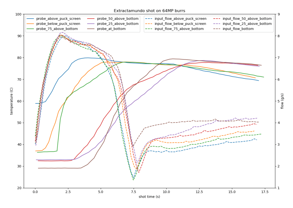
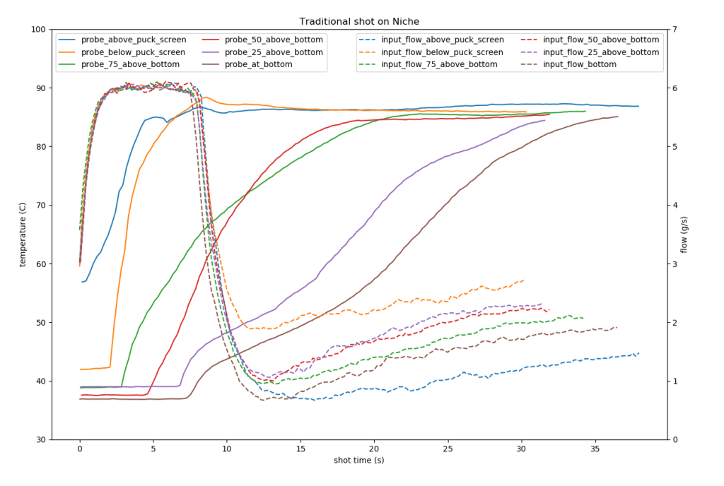
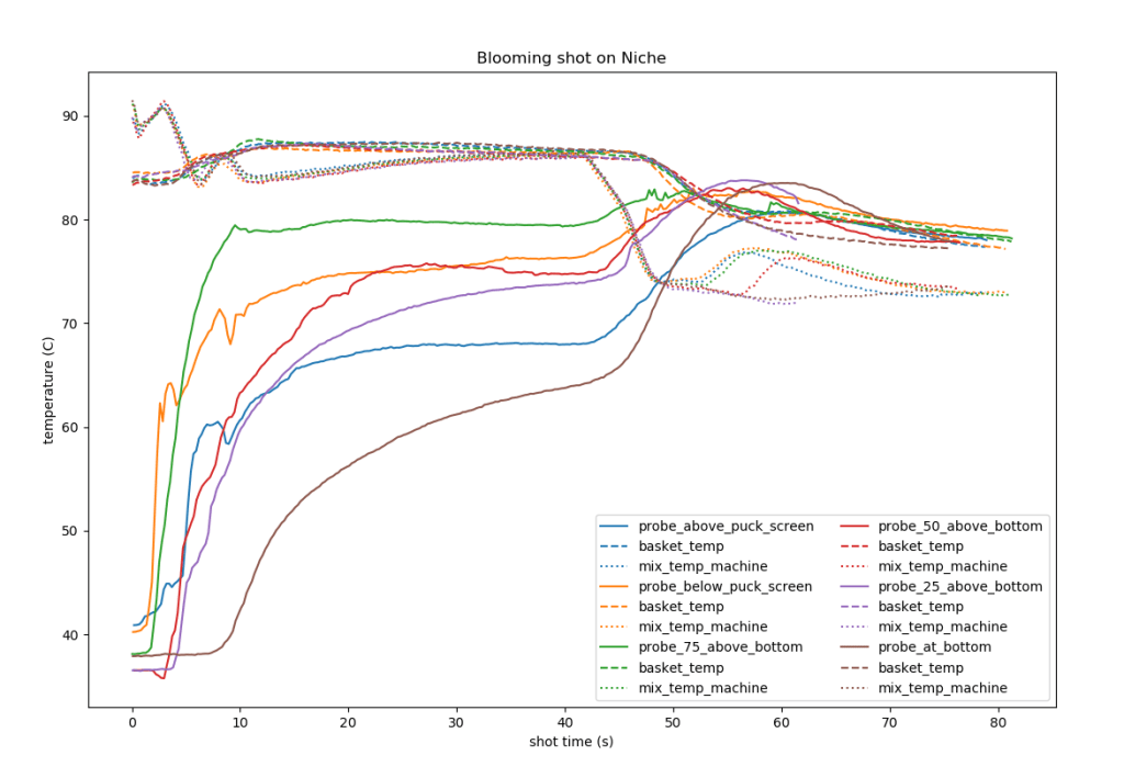
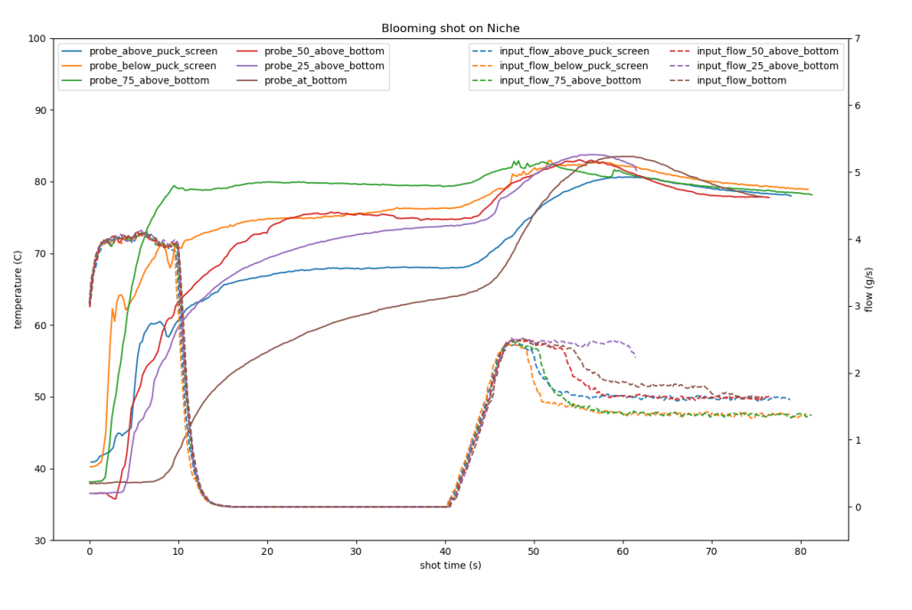
For each shot type, you’ll see two plots – one containing the probe temperature for all six heights along with the corresponding basket_temp and mix_temp (this is the temperature of the “fresh” water being sent out to the group after the firmware has taken necessary action to mix hot and cold water in the right amounts to try and reach the target temperature as soon as it physically can); and the other containing flow rate data. In all the plots that follow, temperature has been plotted in solid lines.

So how bad is it?

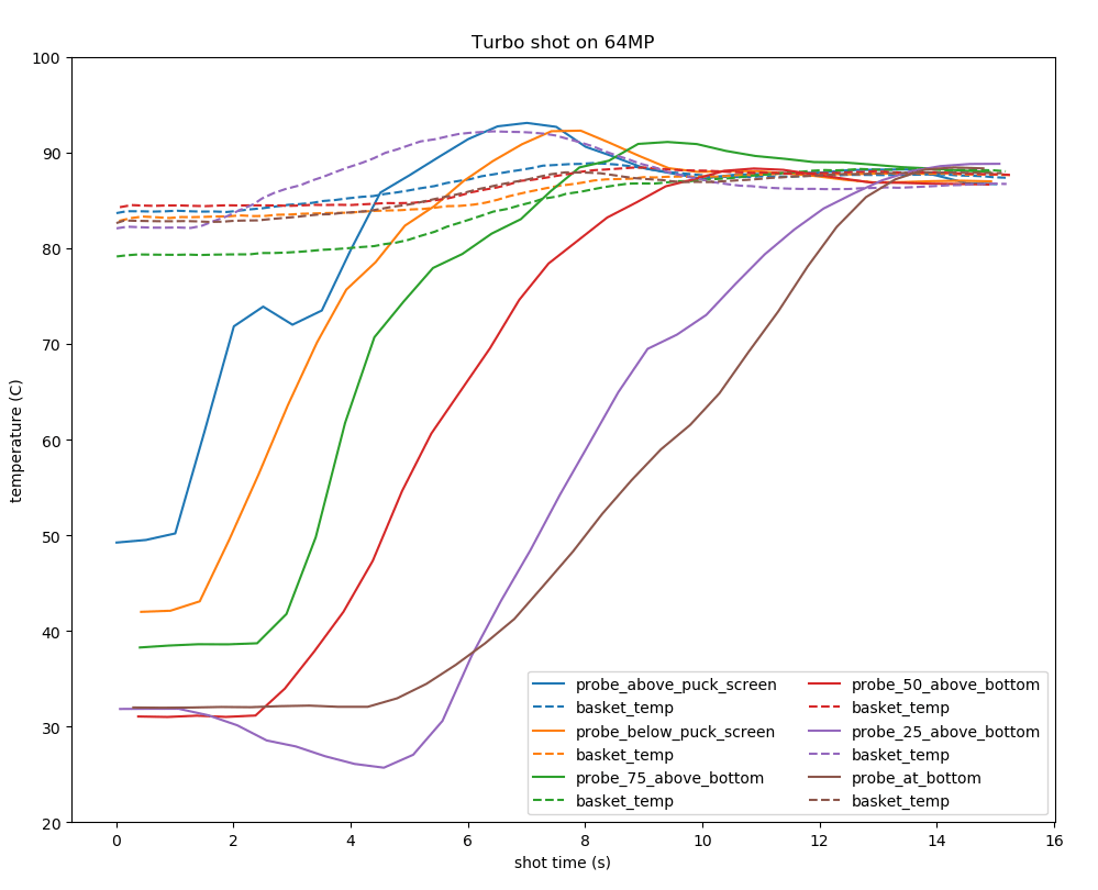
Depends on who you ask. A lot of industry professionals who have suspected this won’t be very surprised (although I’m curious if they’re amazed at the extent of it in some of the cases listed above). If you focus on the temperature plots and temporarily forget the flow rate aspect, you’ll notice (while being appalled) at how wide the difference is at a given point in time between the top and bottom of puck. In fact in case of the traditional shot, if you were to stop it at the 30 second mark as is usual, the bottom of the puck will have barely reached the same temperature as the top of the puck. This is also somewhat the case for regular turbo shots if you were to stop the shot at 15 seconds (the bottom of the puck in this case having spend a bit more time at the same temperature as the top of the puck).

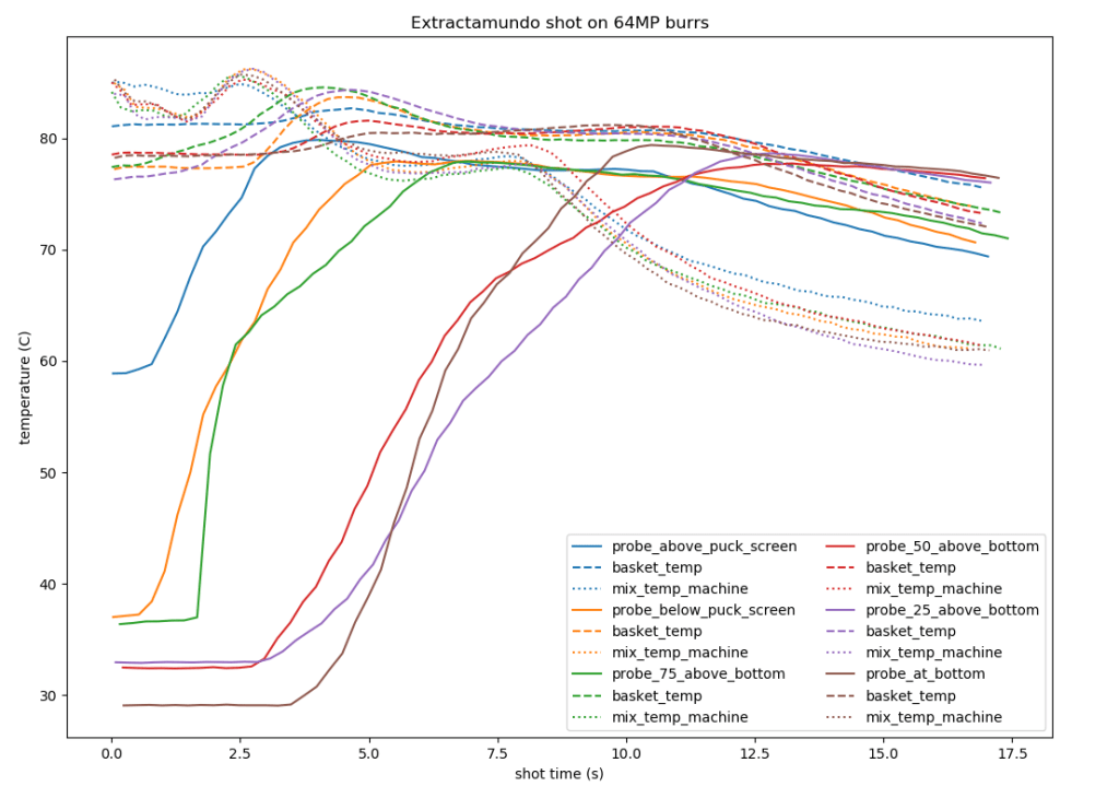
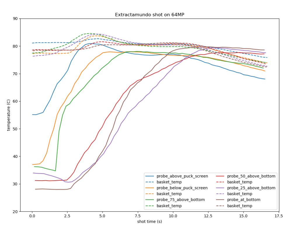
On the other hand, JoeD’s approach of a declining temperature during turbobloom (Fig 2a) does seem seem to make more of the puck extract at closer temperatures, if not similar (shoutout to Christopher Feran who first pointed this out to me). I also thought this would be a good chance to test Scott Rao’s claim of blooming a puck for 30 seconds resulting in more even temperature throughout the puck, and indeed from Fig 4a it does seem like the puck seems to start at a delta of 20 C once pressure starts ramping at around the 40 second mark as compared to a 45 C delta in Fig 3a that it cannot seem to recover from in case of a standard shot. I’m intentionally referring to the delta when pressure ramps because I chose to also induce declining temperatures in the blooming shots (as has been my modus operandi for blooming shots over the last year). Note that I have used a customized adaptive version of the blooming shot that “adapts” flow rate based on when it detects a pressure decline (this allows it to settle to a flow rate based on behavior induced by the probe’s channel).

Elephant in the puck named Flow

So how do we improve our plots with the flow rate variance in the data we collected. Well, a very interesting thing about temperature is that if you introduce any sort of change in temperature in the DE1, any difference in flow rate affects the rate at which that temperature changes. If you look carefully at figures 2a vs. 2b and figures 4a vs. 4b, you’ll notice that the phases for which I induce a temperature decline, the rate at which it drops temperature (both basket_temp and mix_temp although in reality the former is a consequence of the latter) is proportional to the flow rate at that point in time. So to normalize temperature vs. flow rate to some extent, I assumed the median flow rate in a given category of shots to be the reference temperature, which in turn meant that the basket temp is assumed to be the same for all shots in a given category. I then took the difference between the original shot’s probe temperature and basket temperature, and re-applied the same differential to the new reference temperature for each shot in a given category to get the normalized probe temperature.

Note – a more accurate way of doing this would be to pull several shots for each location of the probe, for a each type of shot, for a given coffee, from a given roast batch, in such a way that it covers a range of flow rates applicable to that shot category, thus enabling us to get a more accurate differential between probe temperature and basket temperature for each probe location. If anyone has say five kilos of coffee they want to donate for this cause, feel free to email me.

Here’s how the somewhat normalized probe temperature plots look like:

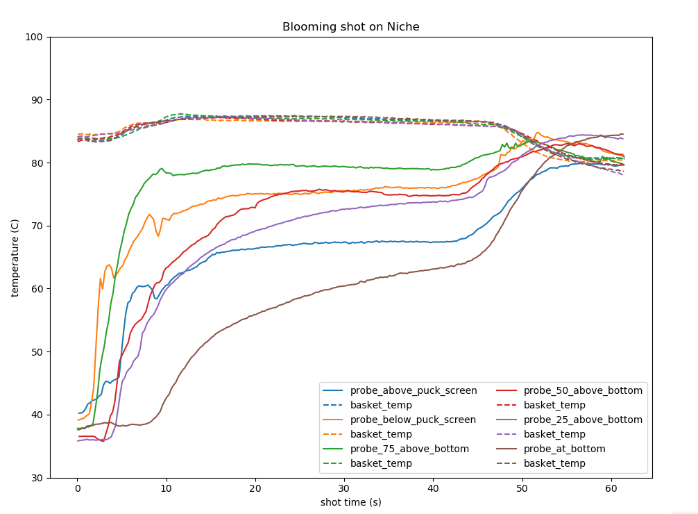
If you look closely, upon normalization, the extractamundo shots have their puck bottoms eventually going a tad higher than some parts of the puck that have started trending lower. Also note that in all cases (except blooming shots where the probe above puck screen showed anomalous behavior and therefore should be ignored), the probe below puck screen seems to lag the probe above puck screen by at worst a second, indicating that thermal loss to the screen is less consequential than other thermal discrepancies in the puck.

A temperature history of water

I kept thinking a bit more about what Christopher (who you may have heard talking about a more green shade of coffee, also happens to have an extremely intricate understanding of coffee extraction; and also roasting) had said – that it seemed like profiles with intentional temperature decline seemed to have more parts of the puck extract at the same temperature. But how can one really tell? Even though I placed probes at 6 different locations (well 5 in the puck, one above the screen), how could one make an estimate of the extraction temperature of every unit volume of water flowing through the puck? If I were to use the normalized flow rate above, and pick certain points in time once water starts dripping out, for every time instant I choose, I have a corresponding flow rate (bless Ray Heasman and his flow modeling). If I were to then assume that an espresso puck’s liquid retention ratio (weight of water retained by coffee grounds) during extraction is 1:1 (i.e. 18g of water for 18g of coffee), then for a flow rate of say 2 mlps, those 18 ml (assuming no added soluble weight for the sake of simplicity since we’re dealing with input and not output flow rate) will take 9 seconds to traverse through the puck. Which means for the four slices we can divide the puck into based on the five probes, every 4.5 ml for a given slice gets replenished every 2.25 seconds. Looked at another way, if the flow rate for a unit volume of water exiting the puck is 2 mlps, 2.25 seconds ago the same unit volume was being measured by the probe sitting 25% above puck bottom, and can therefore be assumed to have been at that temperature 2.25 seconds ago (I acknowledge that the flow rate may not have been sustained at 2 mlps for the duration of those 2.25 seconds, but we would need more slices for more accuracy). Besides the temperature information, we also have flow information for the probe 2.25 seconds in the past. If for some reason the flow back then was slower, say 1.5 mlps, we can assume that the same unit volume took 3 seconds to traverse through the previous slice, and we now have the temperature for the same unit volume of water from three more seconds ago from the probe sitting 50% above bottom.

If you now apply this to a given number of points at the output of the puck (bottom most probe), and back-calculate temperature all the way to the probe above the puck, you now have the temperature journey every unit volume of water takes when traversing through the puck (unit volume in this case more accurately means the volume of water that flowed through the puck, which is a tad less than output weight, divided by the number of traces for that given plot).

This is how the temperature journeys look:

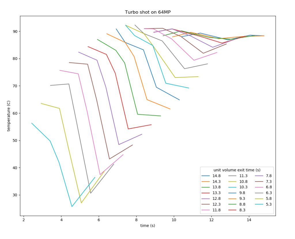
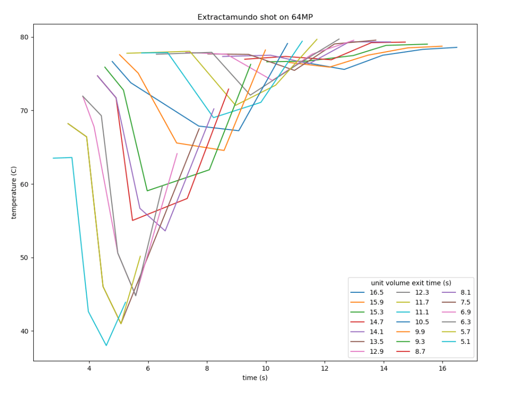
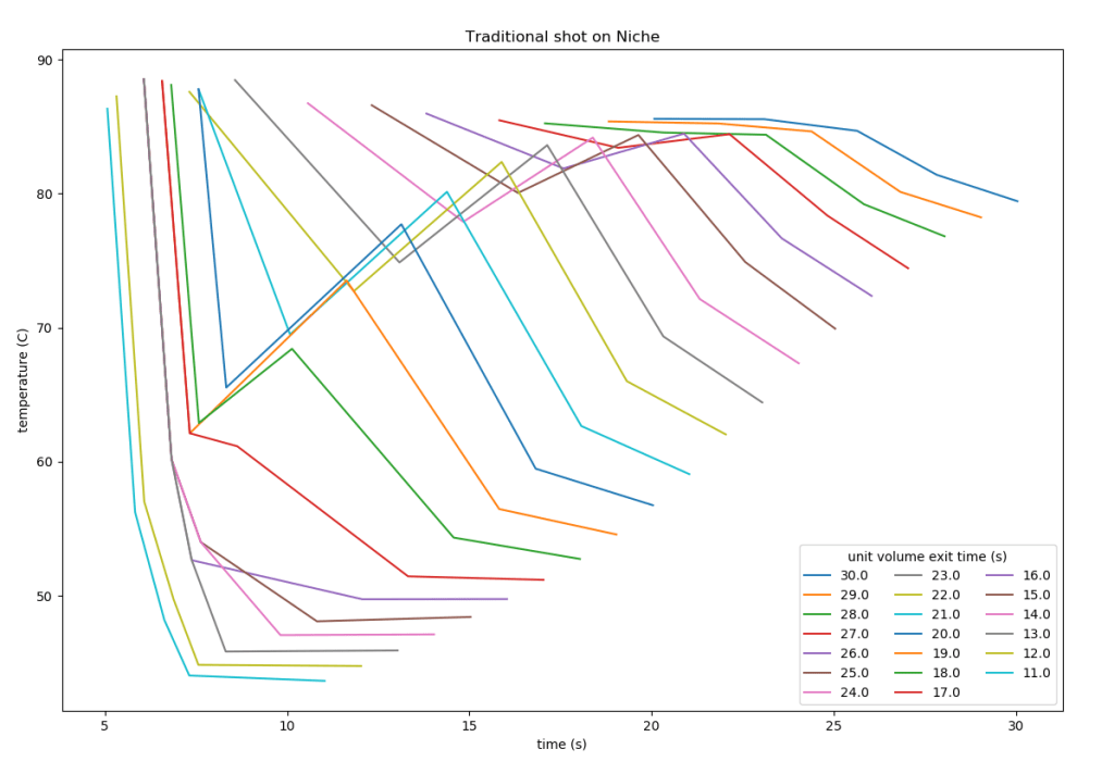
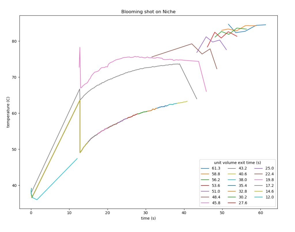
As is quite clearly visible, in instances where temperature declines were induced, a unit volume of water seems to have traversed the puck with less fluctuation in temperature once pressure had ramped (indicated by when flow flattens out or has a relatively gradual increase in figures 1b, 2b, 3b, and 4b).

Does it get any worse

I was chatting a few days ago with Michael Cooper of Quantitative Cafe (if you haven’t read his posts you should get yourself up to speed on his spectacular content). Cooper happened to be talking about viscous fingering in an espresso puck and how the top of the puck loses solubles almost instantaneously. While we wait for his (and Shay’s, who was probably the first to think of it in context of espresso) blogposts on the subject rather impatiently, one of the major driving forces of this phenomenon occurring in an espresso puck is the difference in viscosity between the top and bottom of the puck as the puck extracts. Supposed evidence of viscous fingering is the dark spots one can see at the bottom of a puck post-extraction (dark regions correspond to regions that have extracted less than the lighter regions). Imagine then how much more severe this phenomenon can become if extraction at the bottom of the puck is hindered even further due to consistently lower temperature than the top of the puck.

Add to this that if we were to assume channeling is already happening in the upper half of the puck due to soluble depletion (where by channels I’m referring to localized pathways of lower tds that allow higher water flow). If Jonathan Gagné’s recent post on astringency is any indication, continuing to keep the top half of the puck that has channels exposed at higher temperatures might play into hands of astringent compounds that tend to be soluble at higher temperatures. You may find a brief mention of declining temperatures in that post (although I would politely disagree on a tiny aspect that depending on the grinder and a given coffee and of course profile, the extent of decline can do anything between extremely vibrant cups on narrow distribution grinders with a steep decline to creating unbalanced taste profiles in case of wide distribution grinders like Niche that may benefit from a less steep decline).

Is the battle lost?

Here’s the thing – an espresso puck is and will probably always be its own worst enemy. But as for the issue of this drastic temperature delta across a puck, we are also looking at some possible solutions (which have also been plotted above). There are a couple of other approaches I would like to comment on but am skeptical they make enough of a difference to mitigate this issue sufficiently, if at all. One is grinders with heating elements – I would be curious to see results of a similar (preferably better) experiment demonstrating a tangible reduction in top vs. bottom delta. The other is portafilters and/or baskets with increased thermal mass. Besides the possibility that water entering the portafilter will be losing heat to sustain the larger thermal mass’ temperature (or more accurately trying to bring equilibrium, whatever temperature that eventually results in may not be the target temperature), thus further taking away from what could have been supplied to the bottom of the puck. In addition, a reduced dose may not mitigate it much either (if the probe placed 25% above puck bottom is any indication), not to mention the usually finer grind needed to build the same puck resistance increasing possibility of clogging.

I hope more folks test puck temperature gradient on their own machines. I’d be curious to know if they see a similar trend.

Acknowledgements

• Christopher Feran: for pointing out that declining temperatures can cause the puck to extract at a more even temperature
• Michael Cooper: for generously sharing his plots of soluble gradient across a puck and facilitating my thought process on this topic
• Collin Arneson: he was the first person I know who stuck a probe on the outside of a basket and said (and I paraphrase), “Y’all are not gonna believe this!”. That may have unconsciously incepted this experiment.

If you have enjoyed reading this post, consider donating to NOT me, but the hourly coffee worker by donating to GoFundBean

Subscribe to keep your pocket updated with coffee science.